How to Use XLOOKUP in Excel {With Examples}

Microsoft has announced the rollout of XLOOKUP – a powerful new function designed to address many of the known limitations of VLOOKUP. 

What is XLOOKUP

The XLOOKUP function searches a range or an array, and returns an item corresponding to the first match it finds. If a match doesn’t exist, then XLOOKUP can return the closest (approximate) match.

How it XLOOKUP works

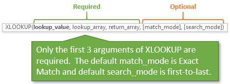
Here is the signature (arguments) for XLOOKUP:

=XLOOKUP(lookup_value, lookup_array, return_array, [match_mode], [search_mode])

It looks a bit scary at first, but only the first three arguments are required. The last two in [square brackets] are optional.

Note: The formulas will only work if you are on a version of Excel that supports XLOOKUP. Currently a portion of users on the Office 365 Insiders Fast channel.

Pros or Advantages of XLOOKUP

Here is the list of advantages for XLOOKUP that I shared in the video above.

1. Defaults to exact match.
2. It only requires three arguments, instead of four for VLOOKUP or INDEX MATCH.
3. Works both vertically and horizontally.
4. One function instead of two, compared to INDEX MATCH.
5. Can do partial match lookups with wildcard characters (4th argument = 2).
6. Can do lookups in reverse order (5th argument = -1).
7. Returns a range instead of a value (advanced nested formulas).

Cons or Drawbacks of XLOOKUP

There are also a few potential issues to be aware of.

1. Additional [optional] arguments can make the function look overwhelming to new users.
2. Returns a #VALUE! error if the lookup and return arrays are not the same length. I explain this in the video above.
3. It can be time-consuming to select two ranges with the mouse, especially when you have thousands of cells in the arrays.
4. You must remember to make both the lookup and return ranges absolute references (F4 on the keyboard) if copying the formula down/across.
5. You must use nested functions to do a 2-dimensional lookup. Can use two XLOOKUPs or INDEX MATCH.

Social Media Response on XLOOKUP :